10 expert tips for better Houdini FLIP fluid simulations
FuseFX artist Kevin Pinga’s current VFX reel shows Houdini’s power to simulate real-world fluids like smoke and liquids. Follow his 10 production-proven hacks to create faster, more flexible FLIP fluid simulations.
Houdini provides a robust set of tools when it comes to simulating fluids. However, making fluids look realistic is a particularly challenging task, particularly for broadcast work.
With TV shows now depending heavily on visual effects, delivery deadlines are getting tighter, yet quality expectations are comparable to those for effects seen in feature films. The pressure is on the artist to make sure a shot makes it to final before it is aired, which in most cases is only days (sometimes hours!) away.
Over the past three years, I have delivered fluid simulation work for TV shows such as The Walking Dead and Castle Rock through multiple studios, including Ingenuity Studios, FuseFX and Luma Pictures. I have also contributed FX work in music videos for artists such as Taylor Swift, Billie Eilish and Maroon 5.
Through these projects, I’ve collected some hacks in my toolbox when it comes to simulating fluids with Houdini’s FLIP solver. These tips and tricks can help you manage your fluid simulations more efficiently when trying to deliver fluid shots in a timely manner, while still maintaining a high level of quality.
The tips are aimed at artists familiar with the FLIP solver, so if you’re starting out, try SideFX’s own tutorials. The images in the article have been scaled down for the web, but you can download the originals here.
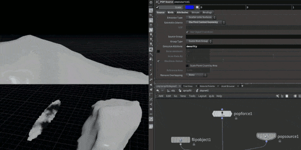
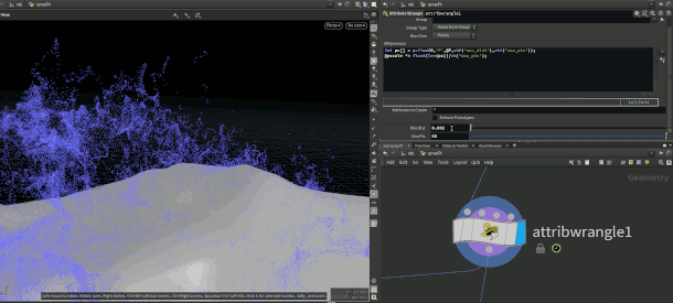
Sourcing fluids with POP Source provides familiar emission, activation and velocity attributes.
1. Source fluids with POP Source, not FLIP Source
The default way of sourcing fluids for FLIP is to use a FLIP Source node, which essentially creates a VDB that is read in by the Volume Source node in DOPs. This is what you get automatically when using the shelf tools.
While this method works fine when you’re sourcing from a large ambiguous shape, it can get quite resource-heavy and time-consuming. Increasing the resolution of your VDB to get accurate more accurate sourcing can slow things further, before you even get to the simulation phase.
Instead, I like to use regular polygon-based SOP geometry directly with no conversion to VDBs. This source can be read in by the POP Source node wired into the Sourcing input of the FLIP solver itself, in the same way that you would import a source for a regular particle simulation.
The controls on the POP Source node are also much more intuitive. Most artists should already be familiar with them through their time working with regular particles. Particle count can be controlled and monitored in a much more predictable way, independent of the Particle Separation of the FLIP object itself.
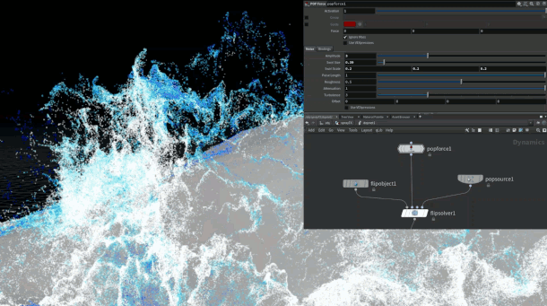
Adding a small amount of noise with a POP Force node goes a long way towards detailing FLIP simulations.
2. Use POP nodes with FLIP fluids
Something that junior artists forget is that FLIP is essentially a series of POPs with some volumetric advection steps in between. However, the base itself is just particles, which means that all the POP nodes in DOPs can be used for FLIP fluids! This is why we were able to source using the POP Source node in the previous tip.
The POP Force node is a staple for creating interesting motion when working with regular particles. So why not use it with FLIP fluids too? Using it to introduce even a small amount of noise can create a more appealing-looking fluid. Low-frequency noises can also be useful for creating detail without having to increase your particle count or particle separation. (Be careful not to add too much noise, as this can cause your simulation to look unrealistic.)
Another POP node that is useful in FLIP simulations is POP Speed Limit. Coupled with a POP Drag node, it works great for controlling high-velocity particles that can otherwise go out control.
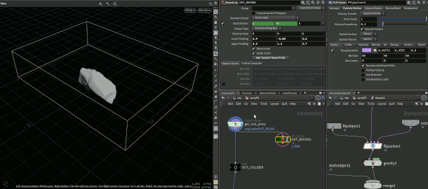
Referencing the parameters in Bounds qL helps to set simulation limits.
3. Use Bounds qL to set your FLIP limits
The Bounds qL node is a very nifty tool that packs in many simple but useful features. It comes as part of a larger open-source Houdini toolset called qLib. In most studios, qLib is installed by default, as its development is driven by real production work. If you don’t have it in your personal production environment, it can be easily be installed by following the instructions on GitHub.
I use Bounds qL primarily for setting my volume limits for FLIP and Pyro simulations. This is a step up from the standard Bound node as it includes an option to create bounds based on an animated input.
The feature that I find most useful is the Output: Values checkbox, which unlocks the values of the size and center of the bounding box. These values can then be copied to any parameter in the FLIP solvers’s Volume Limits tab, or any other operations that require a bounding box. Having centralised bounding box info can avoid user error and helps in creating more procedural setups.
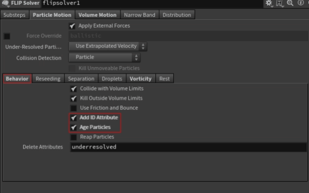
Enabling extra FLIP attributes: like a lot of things in Houdini, the fix is only a few checkboxes away!
4. Enable useful attributes in the FLIP solver
There are some parameters on the FLIP solver that I like to turn on in most of my FLIP sims. The three main ones are ID, age and vorticity. They can be used to make post-simulation tweaks, as we shall see in the next tip, and can all be found in the FLIP Solver under the Behavior and Vorticity tabs, as shown above.
Most artists are already familiar with the ID attribute and how powerful it can be. Your data size might take a small hit for caching an additional attribute, but it’s always a good idea to have that information available.
Enabling the age attribute via the Age Particles checkbox (which also exports the life attribute) makes it possible to control how a sim looks over time, especially if you have a source that is constantly emitting.
The vorticity attribute is handy for sourcing secondary simulations like whitewater and is great for manipulating shading.
A simple VEX wrangle to adjust particle size based on the density of the point cloud.
5. Do post-simulation tweaks to salvage failing sims
There is a tendency to rely heavily on the output of a FLIP simulation as a final result. While this an ideal workflow, due to time constraints, you don’t always have the luxury of resimulating to fix problems. In cases like these, running post-simulation tweaks on the FLIP particles themselves can help ‘salvage’ the sim.
For example, one of reasons to add the ID attribute is that it enables you to use the Retime node to retime a sim. There have been times where I have forgotten to turn on this checkbox, only to find that the only note I received on the shot was ‘Make it slower by 80%’, meaning that I had simulate everything again.
Another common problem that I encounter when running mid-res simulations is that the size of the liquid droplets is good in high-density areas of the simulation, but too big in sparser areas. In cases like this, a simple wrangle using the pcfind: function can help mark sparse areas and lower their pscale value.
Here’s the code snippet used in the wrangle:
int pc[] = pcfind(0,'P',@P,chf('max_dist'),chi('max_pts'));

@pscale *= float(len(pc))/ch('max_pts');
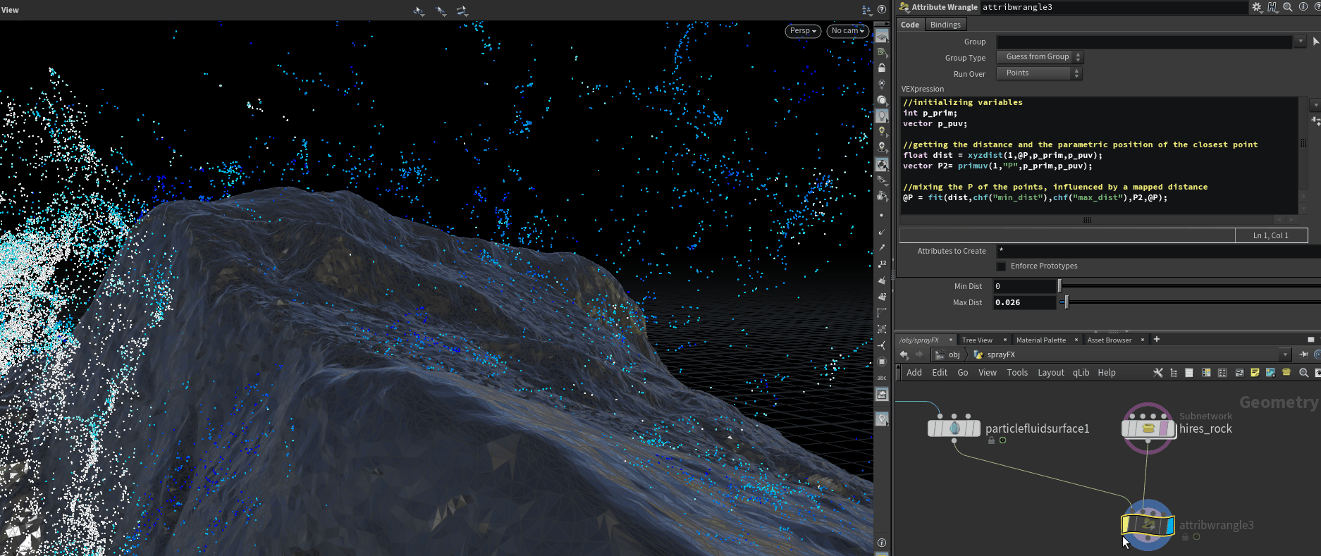
Using xyzdist() and primuv() to push particles towards the collision surface.
6. Use xyzdist to handle high-resolution collision surfaces
This is another post-simulation tweak, but I find xyzdist() to be so useful that it deserves a point on its own. It is by far one of my most-used functions, along with primuv().
In a VEX or VOPs context, xyzdist() calculates the distance to the closest interpolated point on a surface. When combined with primuv(), you can extract any attribute from the parametric UVs of the object!
In the case of the example above, the position of the high-resolution collision surface is extracted and used to push particles towards the surface. In some cases, you can also run this directly on the meshed surface itself, especially in shots where the collision surface is see-through (for example, pouring liquid into a clear glass). Make sure you clamp the distance to a really small value to speed up calculations!
Here’s the code snippet used in the wrangle:
//initializing variables

int p_prim;

vector p_puv;

//getting the distance and the parametric position of the closest point

float dist = xyzdist(1,@P,p_prim,p_puv);

vector P2= primuv(1,"P",p_prim,p_puv);

//mixing the P of the points, influenced by a mapped distance

@P = fit(dist,chf("min_dist"),chf("max_dist"),P2,@P);
In production, a more practical usage would be use a lower-resolution collider during simulation, and then run this function in a post-simulation wrangle to make the fluid look like it’s interacting with a high-res collider.
I’d highly recommend checking out Henry ‘toadstorm’ Foster’s blog post for a more detailed explanation of xyzdist() and primuv().
A simple method to correctly blast away problematic particles via ID attributes.
7. Kill problematic particles with ID
This is a simple yet effective trick when you have a simulation that is 98% close to being final, but where the remaining 2% of particles are just not working. If you stored the ID attribute mentioned in the previous tips, you can use it to blast away the problem particles. Without ID, you wouldn’t be able to mark the correct particles for deletion as the point count changes from frame to frame.
The best way that I have found to do this is to go into point selection mode and hit [9] on your numpad. This brings up the Group Selection pane. To select by ID, click on the gear icon and select Attributes > id. Now you can simply select the particles you want to remove in the viewport and hit [Delete]. A Blast node will be generated automatically referencing the point ID instead of the point number.

Turn up surface oversampling to fill sparse areas of a simulation.
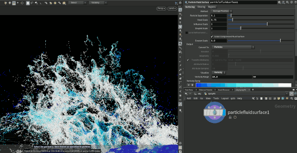
8. Use reseeding to beef up sparse regions
In production, most of the development work on simulations is done using a mid-resolution container. Sometimes, you may end up with a mid-resolution FLIP sim that has hit all the notes you need to hit, but which doesn’t have enough particles for it to look correct when meshed for a final render. You lower your Particle Separation setting in the FLIP solver (which increases resolution and particle count), submit your simulation to the farm, and go home to enjoy whatever is left of your weekend, only to come back the next morning and discover the simulation now looks completely different!
In cases like this, I prefer to turn up the reseeding parameters instead of changing my particle separation. By default, reseeding is already turned on, but cranking up the Surface Oversampling parameter can help increase particle count in sparse areas by spreading out the particles. This way, you get to keep the general look of your simulation but have enough particles to avoid the meshed fluid looking like Swiss cheese.
Check out this excellent video from Dave Stewart to see the workflow in action.
Rendering the original FLIP sim directly as whitewater.
9. Use the original FLIP sim directly as a different element
One of my goals when working with fluid simulations is to maximise the usage of the original FLIP simulation. This includes using it directly as whitewater.
The traditional way to create whitewater is to simulate the FLIP fluid, then run the Whitewater solver on top of that. However, the second step isn’t always necessary, particularly for fast-moving fluids like splashes and water jets (think a broken fire hydrant or underwater in a hot tub – and yes, these are shots from real projects!). In addition, it can be quite tricky to get the fluid to look right when meshing the particles.
Instead, what you can do is take the FLIP sim itself and render it directly with a whitewater shader. You can either render the particles themselves, or rasterise them to a VDB and render the result as a volume. I use a mixture of the two techniques depending on what looks best for a shot. The whitewater shader that is created automatically when using Houdini’s ocean tools works quite well for rasterised particles.
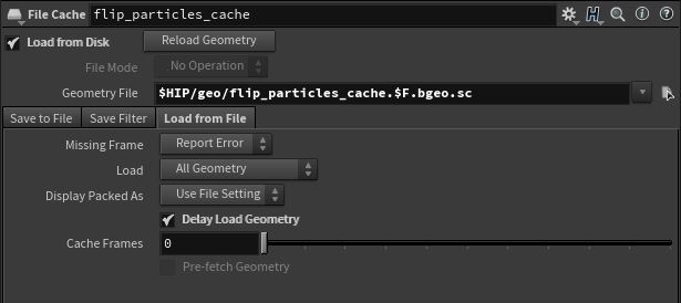
Use the Delay Load Geometry checkbox in the File Cache node to speed up work on high-res sims.
10. Optimise the sim and caches
One of the challenges with high-resolution FLIP sims is dealing with the large amounts of data they generate. A common practice is to delete all the attributes that you don’t need before caching any part of a simulation.
Another thing that you can do to help reduce your memory footprint is to cull the particles outside the camera’s frustrum. There are many methods to do this in Houdini, so use whichever you prefer.
Additionally, if you have geometry that is ready to be rendered, it is a good idea to cache it out and have the Delay Load Geometry checkbox turned on. Instead of having Mantra embed the geometry in the IFD file, it will be referenced to the file on disk instead. This will help reduce load times and also drastically reduce both IFD generation times and file size. Helpful if you have a render farm and don’t want to bog it down!
 About the author: Kevin Pinga is a Los Angeles-based FX artist who has worked on award-winning films and TV series including Spider-Man: Far from Home, which recently won the AACTA Award for Best Visual Effects. Additional projects include AMC’s The Walking Dead, Brooklyn Nine-Nine, and music videos for Taylor Swift and Billie Eilish. Visit Kevin’s website.